| name | height |
|---|---|
| Emma | 1.6 |
| Rani | 1.4 |
| Sven | 1.5 |
BI for beginners (session 5)
Power BI
beginner
Previous attendees have said…
- 14 previous attendees have left feedback
- 100% would recommend this session to a colleague
- 100% said that this session was pitched correctly

NoteThree random comments from previous attendees
- Really useful explanation of breaking down large datasets into useable tables within Power BI
- I think this would fit really well as session 5 of the beginners sessions. It’s a good way to consolidate what is covered in the other 4 and highlight ways in which to practically use power BI in “real” life. Thank you!
- Good to be able to compare how data can be compressed in different ways but give the same outcome. Shows you don’t need reams of repeating data to get good quality!
NoteSession materials
There are two Excel datasets for this session
Session outline
- In this session, we’re going to think about data modelling for Power BI
- we’ll start with a sub-set of the GP data we were working with over the past couple of sessions
- as we’ll see, the simplest (and most Excel-like) way of holding that data isn’t a natural fit for work in Power BI
- we’ll use the model to explore that data
- we’ll introduce the idea of a star schema as the usual way that you’ll need to organise your data for Power BI
- and we’ll conclude with a practical exercise in Power Query showing how to turn flat data into star schema’d data
Setup
- download both datasets (.xlsx full data and .xlsx split data) to somewhere sensible on your computer
- connect to the full data Excel file, and load the single table
- recreate a simple starting dashboard as a warm-up exercise

What’s the problem?
- this data is held as a single flat file
- while easy to understand, it’s highly repetitious: the seven GP practices in Orkney require 25 columns and 112 rows of data - so 2800 values in total
- this causes performance issues (as well as brain-ache)
What’s the solution?
- we can break this data into several related tables
- that reduces repetition and makes the data easier to understand
- this has the useful side-effect of speeding-up Power BI
Jumping ahead: a second bout of data loading
- create a new report
- connect to the .xlsx split data and load all four tables

- have a look at the data - you’ll see that it’s much more concise (582 values in total - so approx a fifth of the size of the full data)
- now inspect your new data in the model
The model
- we should see our data tables as blocks in the model

- there are also connections between some of those blocks
TipTask
- Mouse-over the relationships in the model view
- What’s the difference between
 and
and  ?
? - Now expand the Properties pane
Relational data
- instead of a single complex file, our data is now held as several related tables
- relationships - the lines between the blobs - show how the parts of our data are connected together
- for example, in the practices table, the HB column (which contains the health board code S08000025 each time) relates to the boards table HB column, which contains matching values
- that means that we can use the data from the boards table - like the name of the Health Board - in our Power BI work
Relationships
- you can see details of your relationships in the properties pane in the model view

TipTask
- make sure the practices-to-boards relationship is set to active - take care to click
Apply - re-create your original map using the postcodes from the practices table and the HBName column from the boards table

Creating a relationship
- if you look carefully at the model, you’ll see a missing relationship
- Power BI guesses which columns might share a relationship by looking for identical column names
- but the population table has a different column name from the practices table. Luckily, we can manually create a relationship:
TipTask
- drag the
DataZonecolumn from practices to theDZcolumn in the population table - that should open the
New relationshipdialogue:
- make sure the cardinality is set to
Many to one (*:1), and make the relationship active
Cardinality
- cardinality describes one feature of a data relationship: how many items should we expect at each end of the relationship?
- the simplest case is 1:1. We’d find that where each value is unique. So if we have two data sets like this, showing something like sports players, with their heights in one table and the number of goals they score in a second table:
and
| name | goals |
|---|---|
| Emma | 5 |
| Rani | 8 |
| Sven | 6 |
Think of the values in the name columns as keys that show us which rows of data correspond to each other. Using these names as keys, we’d expect a 1:1 relationship between the tables. Each key value is unique in each table, and so we’ll get exactly one value for Rani’s goals and height, for example. If we had several different rows for each player’s goals…
| name | goals |
|---|---|
| Emma | 5 |
| Rani | 8 |
| Sven | 6 |
| Emma | 4 |
| Rani | 7 |
| Sven | 6 |
This would give us a 1:many (which Power BI calls 1:*) relationship, where we’d expect to get several rows from the goals table for each row in the height table.
TipTask
-
add table with
GPPracticeNameandPopulation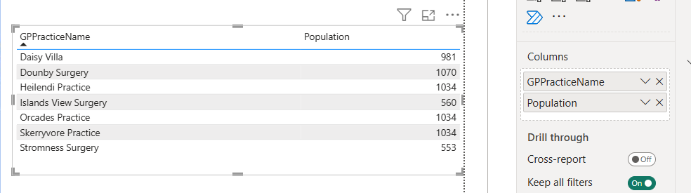
Cross-filter direction
Cross-filtering is the behaviour that you see when one visual filters another visual. For example, if you click on one of the practices on the map, your population table should update appropriately. Similarly, click on the population table, and your map should update too to reflect the selected areas. This type of two-way filtering behaviour is the default, and (slightly confusingly) the cross-filter direction toggle in the Properties pane of the relationship won’t change it.
Cross-filtering should nearly always be one-way to avoid vagueness in your model. But there is one case where it might be useful to demonstrate a two-way cross-filter on a relationship, which is where you want two slicers to filter each other. We’ll demonstrate that using two slicers, with one using GPPracticeName, and the other DZ.
The star schema
If you look at our data, we’ve got a single central table (with the practice details), and then a group of three lookup tables that contain fine-print details about each one of the practices. That’s starting to approximate a star schema
In a star schema, your data is broken into several tables which are joined by relationships. Most of the data is held in dimension tables, which contain data on a theme. For example, our population table above is effectively a dimension table, because it holds all the information about the population in some datazone. That data is organised by primary key - here, the datazone codes in the DZ column - which uniquely identify rows in the table.
Each dimension table is then joined by a relationship to a single fact table. The fact table contains only the unique combinations of the primary keys from the dimensions table. So, if we were star schema-ing our GP data, our fact table would contain the following:
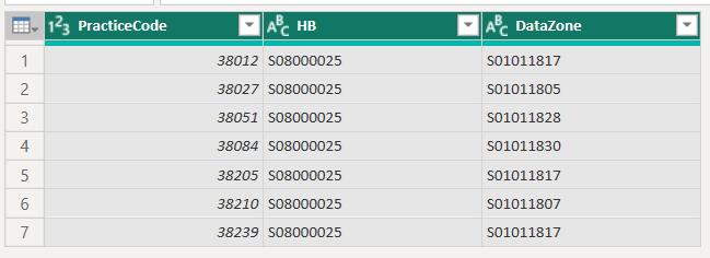
That’s one row per practice, with the unique PracticeCodes in one column, their health board in the HB column - that’s boring because all our practices in this dataset are in Orkney, but would be more interesting and useful if we were dealing with practices from several NHS boards - and the non-unique datazone of each GP practice.
Starring your data
we’ll leave this as an optional section (either at the end of the main session, or as homework) for people who’d like to practice their Power Query
we’ll work through how to transform the flat file into properly Star schema’d data

-
in outline, the steps are to:
- take the full data query and duplicate five times (one per final table)
- rename each query (
main_table,demographics,boards,population,practice_details) - select the columns you need for each table:
- PracticeCode, DataZone, HB in the main table
- PracticeCode through to GPCluster in the practices_details table
- PracticeCode, age_range, n_patients, and Sex in the demographics table
- DataZone, Population, SIMD2020v2_Rank, DZname, and URname in the population table
- HB, HBName, HBDateEnacted in the boards table
- remove duplicate rows in each table
- then check the relationships to make sure the keys and cardinalities match up
Duplicate your query
There are a couple of ways of creating a copy of a query. We discuss these more fully in our intermediate Power BI sessions, but approximately you can:
duplicate a query, which re-creates the whole process from scratch by loading the data from source again. This is slower, because you need to duplicate a lot of work, but makes for fully-independent queries. You can, for example, duplicate a query and then safely delete the original query without causing trouble
or you can reference a query, which takes a snapshot of an existing query. This is faster than duplicating, but means that your daughter query depends on the original query, and if you change the original then your daughter query will potentially change/break too
For this practice session, keep things simple. Create four duplicates of your s05_full_data query, and rename them main_table, demographics, boards, population, practice_details. Don’t try and leave a spare copy of your original data hanging around, because that’ll complicate building relationships later.
Selecting columns
start with the main table. Here, this table will only contain keys, which are the unique values that describe our different GP practices, health board(s), and datazones
the
Choose Columnstool is definitely the most friendly way of doing this selection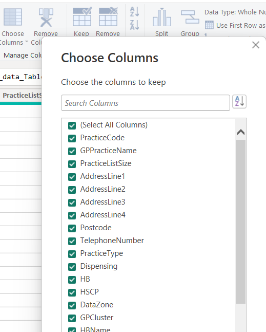
Duplicate rows
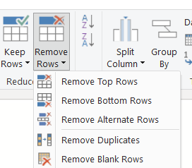
Remove Duplicates function is tricky, because it changes its behaviour depending on the selected columns. If you select a single column, Remove Duplicates will remove any duplicates in that column only and will ignore other columns, meaning that you can potentially miss combinations in your data. So given this sort of raw data, which contains no duplicated rows: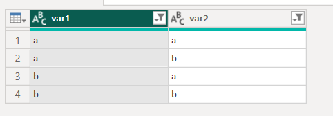
Remove Duplicates on var1 (with the formula = Table.Distinct(#"Changed Type", {"var1"})) will incorrectly remove some rows:

That clearly misses some unique combinations of var1 and var2 in the data. Make sure you select all the columns (ideally using Ctrl + A) before running Remove Duplicates. Note that reading the formula is useful here, because the correct formula (= Table.Distinct(#"``Changed Type``")) doesn’t specify any column names.