Data tidying in Excel
excel
intermediate
NoteSession materials
Welcome
- this session is 🌶🌶 - for intermediate Excel users
- materials can be found on our training pages: tinyurl.com/kindtrp
- you’ll need Excel, ideally M365 desktop to follow along
- you’ll also need the sample data
Session outline
- understanding tidy data
- a practical introduction to making tidy data
- tables
- autofill
- text to columns
- validation, manual reshaping, and PowerQuery demo
Understanding tidy data

- tidy data is not specific to Excel (e.g. this session is partly adapted from chapter 5 of R for Data Science)
- if we tidy our data, we’ll be able to compute it
- standards for tidying data help make for safe and effective analysis
Values
-
valuesis the word we use to describe each bit of information in an Excel spreadsheet. Some examples: - a date, like
2024-06-28 - a number, like
11.2 - a name, like
NHS Grampian - a cost, like
£12.50 - …
- each value should have its own cell
Entering values
- how would you enter this data:
2018, 2019, 2020, 2021, 2022? - please now:
- open Excel
- start a new workbook
- add a column header
yearin cellA1 - then add each of those five values in the five cells underneath (down to
A6)
More values
- we’re going to be using some birthrate data from the NRS for this session. We’ll start by adding some birth rate data
- this is given as births per 1,000 women in five year age brackets. We’ll start with 25-29 year old mothers
- please add the header
25-29yrsin cellB1 - here are the values for our five years:
73.4, 71, 66.8, 69.6, 66.7
Tables
- you should keep your new data in a table
-
Insert>Table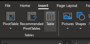
- tables allow you to sort and filter your data
- they also act as a useful ‘container’ (or data structure) for your data
Extending tables
| 30-34yrs |
|---|
| 90.9 |
| 88.6 |
| 83.4 |
| 85.9 |
| 84.4 |
- please could you add some new data to your table showing births for another age group
- you should be able to drag the blue table corner over your new column to extend the table

Autofill
- one last way of adding values: autofill
- drag again to make a new empty column, and label it
difference - in
D2(the first ‘proper’ cell), copy this formula:=C2-B2. This will calculate the difference in birth rates between the two columns - finally, click the small green corner of that newly-filled cell to autofill the column

Back to tidy data
- we’ve now got some data with:
- each value in a cell
- each variable in a column
- here, this is a maternal age bracket
- each observation in a row
- here, this is a year
- we could work through and extend this data by hand, but we’ll now switch over to some supplied data to save all the typing
- errors are common in manual data-entry
- if you can import data, that’s usually better than re-typing it
Many values per cell
- We often find useful data with more than one value per cell
- this can be helpful for humans

- Excel can’t do anything with this data
Exercise one: many values per cell
- find the
Exercise onesheet in the exercise file - try calculating an average for each of the groups
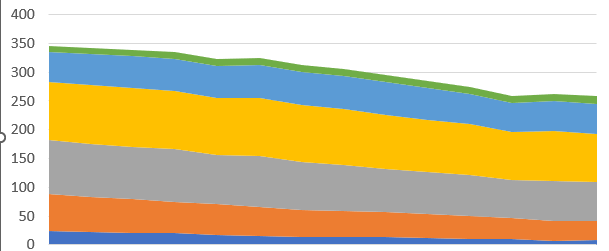
- or, if you’re more confident, try plotting the data
Nothing works!

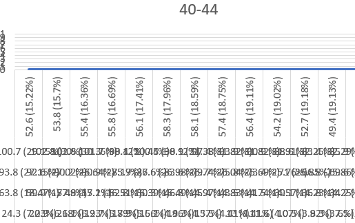
What’s the solution?
- make this data have one value per cell
- we could remove all the percentages by hand - but that’s going to be very slow
-
Text to Columnsgives us a better tool for the job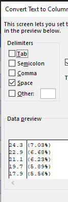
Text to Columns
- select a column
- in the
Datatab of the ribbon, you should find theText to Columnstool
- note that you can keep, or remove, the percentage column. We’ll skip it, to keep things simple
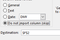
Try working with that data again
Exercise two: transposed data
- sometimes you’ll find data where the columns and rows have been flipped

- that’s slow to fix by hand, but luckily you can transpose it, which swaps rows and columns
- select your data, and copy/paste into a new cell
- then use the transpose option
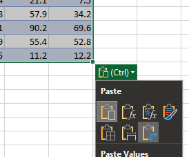
- you might need to fix formatting and labels:

- the
Clear formatsoption might help this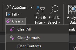
- if you run into trouble, please note that transposing only works on data that is not in a table
Validation and really messy data
- one of the most time-consuming bits of tidying is checking your values
- we’ll briefly demonstrate the data validation tool
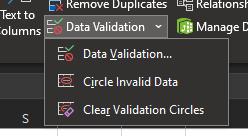
- you can follow-along from the
Demo one (validation)worksheet - this allows you to describe what format you think your data should be in, and then highlights anything that doesn’t fit
- we select the
yearscolumn - then open the data validation tool
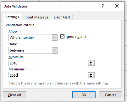
- then set appropriate validation options, so Whole number between 2010 and 2030
- then select
Circle Invalid Data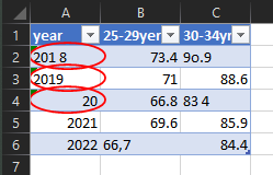
- we can now go through and fix anything circled
Reshaped data
- there are several automated ways of reshaping data that’s not in a tidy format
- we’ll look at the manual way here, but - as it’s horrible - I’d be keen to encourage you to investigate Power Query or Pivot Tables to reshape if this is a regular part of your working day. PQ takes < 10 seconds, PT not much longer
- you can follow-along from the
Demo two (reshaping)worksheet
Manual reshape
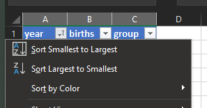
- sort the data by year
- then copy and paste blocks of data, making sure to keep the years aligned

- make sure you then copy the age brackets to label the column
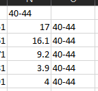
- then delete the spare years columns, and the age brackets
