Dates and times with lubridate

beginner

Published

July 6, 2026

Previous attendees have said…

4 previous attendees have left feedback
75% would recommend this session to a colleague
100% said that this session was pitched correctly

Three random comments from previous attendees

The sessions was useful for grounding us in basic lubridate skills
Nice introduction, examples and practice for using lubridate.
All the content was very relevant. Found the run through a bit quick but I think I picked up most of it. A useful summary of the lubridate functions, thank-you.

About this session

this is a beginner’s introduction to working with dates and times with lubridate
focus on core parsing, get/set, and rounding functions
lots on dates, a bit of date-times, no times

Session resources

Lubridate cheatsheet
R4DS 2e chapter on dates and times
quick primer on ISO8601
there’s also a bit of optional sample data which you can download as a .csv

Why lubridate?

makes some of the simple things easier
- also makes some of the complicated things possible, even though we won’t talk about them here
note that lubridate is:
- not the only way of dealing with dates
- not always the best, but on balance the most consistent, and least quirky tools for dates

Getting started

Open a new Rstudio project
In the console, run install.packages("lubridate")
Once installation has completed, create a new R script and save it
Add library(lubridate) to the start of the script

Dates in R

effectively an integer count of days since 1970-01-01 (basically Unix time)
that means we can convert integers to dates using as_date():

library(lubridate)
as_date(0) # showing the start of Unix time

[1] “1970-01-01”

as_date(20640) # date-of-writing

[1] “2026-07-06”

as_date(-1000) # unlike Excel, R is fine with dates before 1970

[1] “1967-04-07”

as_date(1:3) # vectorised

[1] “1970-01-02” “1970-01-03” “1970-01-04”

class(as_date(1000)) # the date class is in base-R, not lubridate

[1] “Date”

as.numeric(as_date(1000)) # converting back from date to numeric

[1] 1000

Date-times in R

effectively an integer too, but of seconds since 1970-01-01 00:00:00 UTC
this is a pain-point when coming from Excel. Excel dates are days since 01-01-1900, and datetimes/times are decimal proportions of days (so 1.5 in Excel = 36 hours)

as_datetime(0)

[1] “1970-01-01 UTC”

as_datetime(1783327643) # date-time-of-writing

[1] “2026-07-06 08:47:23 UTC”

as_date(-1000) # unlike Excel, R is fine with dates before 1970

[1] “1967-04-07”

as_datetime(1:3) # vectorised

[1] “1970-01-01 00:00:01 UTC” “1970-01-01 00:00:02 UTC” [3] “1970-01-01 00:00:03 UTC”

class(as_datetime(1000)) # date-times are held using the POSIXct class, again from base-R

[1] “POSIXct” “POSIXt”

as.numeric(as_datetime(1000)) # converting back from date to numeric

[1] 1000

as_datetime(2 ^ 31-1) # 32 bit signed int, which might cause a few problems

[1] “2038-01-19 03:14:07 UTC”

Time zones

these date-times have an implicit time zone built-in (which is UTC)
that’s potentially very important for time calculations (e.g. when calculating shifts when the clocks go back or similar)
time zones are also part of base R
we can set the time zone explicitly:

as_datetime(1783327643, tz = "GB")

[1] “2026-07-06 09:47:23 BST”

as_datetime(1783327643, tz = "Europe/London") # equivalent: don't think there are specifically Scottish codes though

[1] “2026-07-06 09:47:23 BST”

you can find your local time zone using Sys.timezone(), and see a list of all time zones (hundreds) using OlsonNames()

Parsing dates

converting dates in your raw data into proper R dates is known as parsing
as_date in our examples above started with a number of days or seconds
if we have dates in our data, we’ll need to calculate those numbers of days/seconds
it’s extremely important. For example…

# spot the deliberate mistake

dat <- readr::read_csv(here::here("r_training/data/lubridate.csv"))

dat |>
  dplyr::arrange(value) |>
  dplyr::slice(1:10) |>
  ggplot2::ggplot(ggplot2::aes(x = date, y = value, group = 1)) +
  ggplot2::geom_point() +
  ggplot2::geom_line()

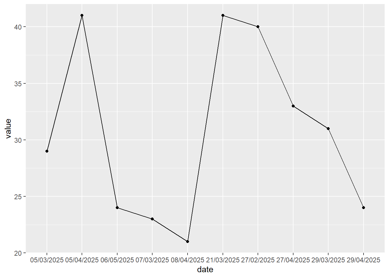
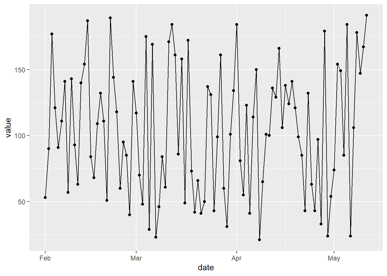
typeof(dat$date)

[1] “character”

make sure that dates in your data are stored as dates/date-times, not chr
str() / glimpse() are your friends here
most functions that accept dates (like ggplot) will mis-behave if you feed them date-shaped-words
- e.g. alphabetically-ordered dates in the plot above
we also often want to be able to calculate with dates
yet this sort of parsing is a pain, because there are loads of inconsistent and ambiguous ways of representing dates

Parsing functions

taking human-readable dates (and date times) and parsing them is where lubridate shines

as_date("2026-07-06") # good for ISO8601-ish dates

[1] “2026-07-06”

dmy("06*07/2026")

[1] “2026-07-06”

ymd("2026__07__06")

[1] “2026-07-06”

dmy_hms("6/7/26 10:32:01")

[1] “2026-07-06 10:32:01 UTC”

# fixed the deliberate mistake
dat |>
  dplyr::mutate(date = dmy(date)) |>
  dplyr::arrange(value) |>
  ggplot2::ggplot(ggplot2::aes(x = date, y = value, group = 1)) +
  ggplot2::geom_point() +
  ggplot2::geom_line()

Inconsistent date formats

date_input <- c("17/5/24", "2024-05-17", "Friday 17th May 2024", "17*May*24", "5/17/2024" )

dplyr::coalesce(dmy(date_input),
               ymd(date_input),
               mdy(date_input))

[1] “2024-05-17” “2024-05-17” “2024-05-17” “2024-05-17” “2024-05-17”

parse_date_time(date_input, orders = c("dmy", "ymd", "mdy")) # similar, but note date times

[1] “2024-05-17 UTC” “2024-05-17 UTC” “2024-05-17 UTC” “2024-05-17 UTC” [5] “2024-05-17 UTC”

What’s the time now?

today()

[1] “2026-07-06”

date_decimal(2024.37534)

[1] “2024-05-17 08:59:11 UTC”

now()

[1] “2026-07-06 11:12:37 BST”

now("Japan")

[1] “2026-07-06 19:12:37 JST”

random_zone <- sample(OlsonNames(), 1)
cat(paste("The date-time in", random_zone, "is", now(sample(OlsonNames(), 1))))

The date-time in America/Rainy_River is 2026-07-06 11:12:37.840098

Get and set

as well as parsing text into proper dates, lubridate has many get/set functions for accessing/changing parts of dates
we’ll show these off using today() to easily generate a date

Years

year(today())

[1] 2026

leap_year(today())

[1] FALSE

quarter(today())

[1] 3

semester(today())

[1] 2

semester(today(), with_year = T)

[1] 2026.2

Months and weeks

month(today())

[1] 7

month(today(), label = T)

[1] Jul 12 Levels: Jan < Feb < Mar < Apr < May < Jun < Jul < Aug < Sep < … < Dec

week(today())

[1] 27

epiweek(today()) # special ways of counting weeks. See  https://en.wikipedia.org/wiki/ISO_week_date and https://www.cmmcp.org/mosquito-surveillance-data/pages/epi-week-calendars-2008-2024

[1] 27

Days

day(today())

[1] 6

wday(today())

[1] 2

wday(today(), label = T)

[1] Mon Levels: Sun < Mon < Tue < Wed < Thu < Fri < Sat

qday(today())

[1] 6

Hour and minute

hour(now())

[1] 11

minute(now())

[1] 12

am(now())

[1] TRUE

dst(now())

[1] TRUE

Set

update(now(), hour = 11, minute = 0, second = 0) # date to date-time

[1] “2026-07-06 11:00:00 BST”

test_date <- dmy("05/06/23")
day(test_date)

[1] 5

day(test_date) <- 11
test_date

[1] “2023-06-11”

Round

floor_date(today(), unit = "week")

[1] “2026-07-05”

round_date(today(), unit = "week")

[1] “2026-07-05”

ceiling_date(today(), unit = "month")

[1] “2026-08-01”

rollback(today()) # last day of previous month

[1] “2026-06-30”

Excel dates

Excel dates start at 1900 rather than 1970

as_date(45429 - 25569) # dirty but effective for dates because it's more human read-able

[1] “2024-05-17”

as_date(45429, origin = "1899-12-30") # better for dates, but note the off-by-one error in 1900-format dates

[1] “2024-05-17”

Excel date times

Excel’s date times are stored as days and fractions of a day
in R, that makes them much more horrible than dates, because we think about date times in seconds, rather than days
do the offset first, to account for the different starting points of the different systems
days have 60 * 60 * 24 = 86400 seconds, so then multiply the decimal part by 86400

as_datetime((46209.43 - 25569) * 86400) # beware the rounding errors though

[1] “2026-07-06 10:19:12 UTC”