stringdist

No feedback found for this session

Introduction

This is an introduction to stringdist which is designed to allow fuzzy matching of text. Install and attach in the standard way:

# install.packages("stringdist") # likely needs compiling
library(stringdist) 
library(ggplot2) # for something fun later

While there are several families of functions in the package, we’ll concentrate on those that focus on the core idea: strings differ, and you can quantify those differences for pleasure and profit. A simple example:

stringdist("thing", "think")

[1] 1

stringdist("thing", "string")

[1] 2

stringdist("thing", "oxpecker")

[1] 8

Once you’ve got an idea about how different you’re okay with your strings being, you can use e.g. a max distance as a cut-off to do work in your code. A simple example of implementing this can be found in the amatch function, which is designed to work like a fuzzy matching version of base-R’s match. We’ll use a and b as variable names to keep aligned with the stringdist documentation. Quick refresher on match:

a <- "the" # take a value
b <- c("this", "is", "the", "thing") # and a vector of possible values
match(a, b) # match returns the index location of your a in your b

[1] 3

Match lets you do useful work with strings - e.g. remove everything before your key word:

b[match(a, b):length(b)]

[1] "the"   "thing"

exemplar: amatch

And now for the amatch version:

a <- "thee" # take a value
amatch(a, b, maxDist = 1) # maxDist = allowable number of typos

[1] 3

amatch(a, b, maxDist = 10) # where several possible values exist, amatch returns the closest match

[1] 3

You can use that in a base-R way to e.g. correct wonky input values:

b[amatch(a, b, maxDist = 1)] 

[1] "the"

Or you might prefer the ain helper:

ain(a, b, maxDist = 1)

[1] TRUE

a %in% b # like a fuzzy version of %in%

[1] FALSE

"the" %in% b

[1] TRUE

Or in a slightly horrid but tidyish way if you wanted to tidy up several different values:

dplyr::tibble(raw_data = c("thi", "ss", "thee", "thung")) |>
  dplyr::rowwise() |>
  dplyr::mutate(is_match = b[amatch(raw_data, b, maxDist = 5)])

# A tibble: 4 × 2
# Rowwise: 
  raw_data is_match
  <chr>    <chr>   
1 thi      this    
2 ss       is      
3 thee     the     
4 thung    thing   

other functions

stringdist, stringsim, and stringdistmatrix

stringdist has a nice toolkit of related functions. stringdist gives you the distance between strings:

stringdist("thing", "think") # gives you the raw distance.

[1] 1

stringdist(a, b) # vectorised

[1] 2 4 1 3

stringsim does the opposite, giving a similarity score between 0 and 1:

stringsim(a, b)

[1] 0.50 0.00 0.75 0.40

stringsim("cat", "dog")

[1] 0

stringsim("cat", "cat")

[1] 1

stringdistmatrix does what you might imagine, returning a matrix of differences. This is largely useful if you want e.g. to pass these scores into something like a clustering algorithm that expects a matrix:

stringdistmatrix(a, b) # same idea, different output: a matrix of differences

     [,1] [,2] [,3] [,4]
[1,]    2    4    1    3

hclust(stringdistmatrix(b))

Call:
hclust(d = stringdistmatrix(b))

Cluster method   : complete 
Distance         : osa 
Number of objects: 4 

plot(hclust(stringdistmatrix(b, useNames = "strings")))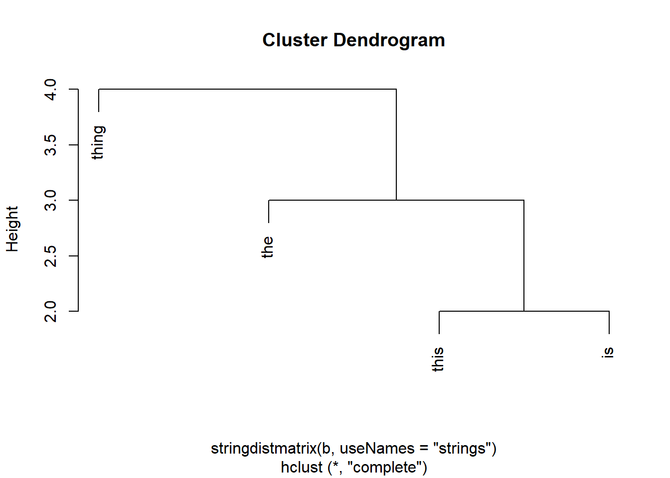

It’s possible-but-messy to take this matrix and tidy it into a tibble:

stringdistmatrix(c("thee", "che"), b, useNames = "strings") |>
  as.data.frame() |>
  tibble::as_tibble(rownames = "a") |> # slightly roundabout conversion to tibble via df to preserve rownames
  tidyr::pivot_longer(!a, names_to = "b", values_to = "stringdist") # useful 

# A tibble: 8 × 3
  a     b     stringdist
  <chr> <chr>      <dbl>
1 thee  this           2
2 thee  is             4
3 thee  the            1
4 thee  thing          3
5 che   this           3
6 che   is             3
7 che   the            1
8 che   thing          4

But probably better/more idiomatic to go:

tidyr::expand_grid(a = c("thee", "che"), b) |>
  dplyr::mutate(stringdist = stringdist(a, b))

# A tibble: 8 × 3
  a     b     stringdist
  <chr> <chr>      <dbl>
1 thee  this           2
2 thee  is             4
3 thee  the            1
4 thee  thing          3
5 che   this           3
6 che   is             3
7 che   the            1
8 che   thing          4

afind, grab, grabl, and extract

afind(a, b)

$location
     [,1] [,2] [,3] [,4]
[1,]    1    1    1    1

$distance
     [,1] [,2] [,3] [,4]
[1,]    2    2    0    3

$match
     [,1]   [,2] [,3]  [,4]  
[1,] "thee" "th" "the" "thee"

afind returns a lot of stuff:

afind(a, b)$location # where in substrings do the search terms start?

     [,1] [,2] [,3] [,4]
[1,]    1    1    1    1

afind(a, b)$distance # how far from the search term is each substring?

     [,1] [,2] [,3] [,4]
[1,]    2    2    0    3

afind(a, b)$match # what's the best matching part of the search term against each substring

     [,1]   [,2] [,3]  [,4]  
[1,] "thee" "th" "the" "thee"

If that’s a bit confusing, grab and grabl are basically replacements for grep(l). grab == grep and grabl == grepl:

c <- c("wig", "win", "banana", "ring")
c[grab(c,  "wig", maxDist = 1)]

[1] "wig" "win"

c[grab(c,  "wig", maxDist = 2)]

[1] "wig"  "win"  "ring"

grabl(c,  "wig", maxDist = 2)

[1]  TRUE  TRUE FALSE  TRUE

c[grab(c,  "wig", maxDist = 3)]

[1] "wig"    "win"    "banana" "ring"  

extract(c, "wii", maxDist=1)

     [,1] 
[1,] "wig"
[2,] "win"
[3,] NA   
[4,] NA   

What do you mean closest?

The really interesting bit: you can play with the method used to calculate distance which will give different results:

hamming

Hamming distance. Number of character substitutions required to change a into b.

amatch("thign", b, maxDist = 1, method = "hamming") # not found

[1] NA

amatch("thign", b, maxDist = 2, method = "hamming") # n subs g, g subs n = 2

[1] 4

lv

Levenshtein distance. Number of del/ins/subs required to change a into b.

amatch("thinng", b, maxDist = 2, method = "hamming")

[1] NA

amatch("thinng", b, maxDist = 2, method = "lv") # as we can now delete

[1] 4

osa

Optimal string aligment. Number of del/ins/subs/swaps required to change a into b:

amatch("think", b, maxDist = 1)

[1] 4

amatch("thign", b, maxDist = 1, method = "osa") # n swaps with g

[1] 4

dl

Full Damerau-Levenshtein distance. As osa, but calculated slightly differently.

amatch("thign", b, maxDist = 1, method = "dl") # can't find a difference with these simple ones from osa

[1] 4

lcs

Longest common substring distance. Comparing longest identical parts of a and b:

amatch("thign", b, maxDist = 2, method = "lcs") # I think roughly = length - common substring

[1] 4

soundex

Distance based on soundex encoding. Used in the phonetic function (see below), but finds homophones:

amatch("thign", b, maxDist = 1, method = "soundex")

[1] 1

stringdist("too", c("two", "to", "oto"), method = "soundex")

[1] 0 0 1

There are also several methods designed to look at q-grams = substring chunks of q characters long, and a group of methods based on the number of similar and different q-grams between a and b:

qgram

This is the q-gram distance:

stringdist("thign", b, method = "qgram")

[1] 3 5 4 0

cosine

The cosine distance between q-gram profiles, which gives you (usefully) a scaled distance of between 0 (identical) and 1 (utterly different)

stringdist("thing", b, method = "cosine")

[1] 0.3291796 0.6837722 0.4836022 0.0000000

stringdist("thing", "fox", method = "cosine")

[1] 1

jaccard

The Jaccard distance between q-gram profiles

stringdist("thing", b, method = "cosine") 

[1] 0.3291796 0.6837722 0.4836022 0.0000000

stringdist("thing", b, method = "jaccard") 

[1] 0.5000000 0.8333333 0.6666667 0.0000000

jw

The Jaro distance (and Jaro-Winkler distance):

stringdist("thing", b, method = "jw", p = 0.2) # correction term

[1] 0.08666667 1.00000000 0.18666667 0.00000000

phonetic

There’s also tooling to deal with the similarity of phonetic spellings. Excellent for e.g. Teams transcripts, if you’re trying to tidy those up:

phonetic("ring")

[1] "R520"

phonetic("wing") # similar sounding strings get similar values

[1] "W520"

phonetic("string")

[1] "S365"

phonetic("strung")

[1] "S365"

a play example: GGC

The KIND network has lots of members from the main NHS body in Glasgow, which is officially known as “NHS Greater Glasgow and Clyde”. That’s a highly variable and abbreviatable name though, leading to over 70 different permutations in common use. Here are some real-ish examples

ggc <- readr::read_lines(here::here("r_training/data/ggc.txt")) # real data

sample(ggc, 10)

 [1] "NHS Greater Glasgow and Clyde"                                   
 [2] "East Dunbartonshire Health and Social Care Partnership (NHS GGC)"
 [3] "NHG Greater Glasgow and Clyde"                                   
 [4] "NHSGGC"                                                          
 [5] "NHS Greater Glasgow and Clyde"                                   
 [6] "NHSGGC"                                                          
 [7] "NHSGGC"                                                          
 [8] "Glasgow Caledonian University & NHS GG&C"                        
 [9] "Glasgow Psychological Trauma Service"                            
[10] "NHS GG&C"                                                        

There’s lots here to play with using stringdist. My two quick examples are to plot a couple of different sensible variants of the name (“NHS GGC”, “NHS Greater Glasgow and Clyde”, “NHSGGC”) methods, and see how many distant results we get:

tidyr::expand_grid(a = c("NHS GGC", "NHS Greater Glasgow and Clyde", "NHSGGC"), b = ggc) |>
  dplyr::mutate(stringdist = stringdist(a, b)) |>
  ggplot() +
  geom_density(aes(x = stringdist, fill = a)) +
  facet_wrap(~a, ncol = 1) +
  theme(legend.position = "none")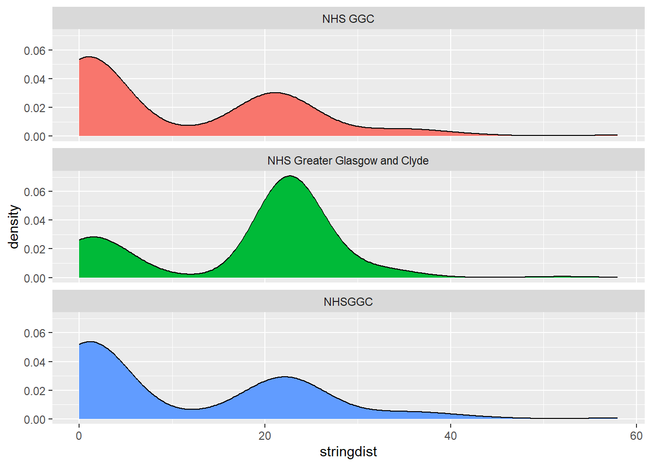

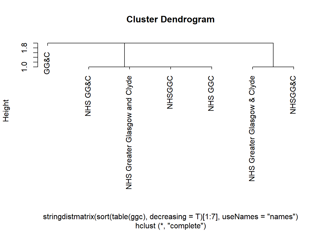
Or to try a family tree (more swishily, a cluster dendrogram) of those terms:

sort(table(ggc), decreasing = T)[1:7] |>
  stringdistmatrix(useNames = "names") |>
  hclust() |>
  plot()