No feedback found for this session
R and SQL
SQL
beginner
NoteAbout this course
- This course is designed as a basic introduction to SQL delivered as live interactive sessions on Teams
- It’s intended as a light introduction for users with good general digital skills (broadly level 2 in the Digital and Data Capability Framework)
- It’s heavily based on the excellent W3 schools introductory SQL course
- If you’re looking for a resource to use to support independent study, W3 schools is a better option than this page
- this material is largely intended to support our live interactive training sessions
- we use posit.cloud for this course. Although that platform is mainly meant for analysts writing R code, we can trick it to allow us to practice our SQL skills
About this session
This session is about using SQL in R. It’s especially designed to help cover three main use-cases:
- Creating SQL databases from R to help when working with big data
- Connect your R project to a (remote) SQL server to access data
- To pre-filter data to streamline later analysis with standard R tools (like dplyr)
The session is an optional extension to our Introduction to SQL course. Unlike the other parts of that course, this session assumes that you have a fair working knowledge of R, and would be capable of reading and writing simple R scripts.
Setup
The setup for this session differs from the other session in the course:
- You will need a free posit.cloud account. Please set this up and check that you have access before the session begins
- Once you’ve logged-in to posit.cloud, if you have an existing project from an earlier session of this course, please return to it and clear the environment
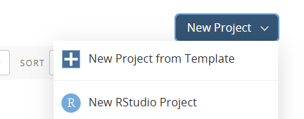
- Otherwise, please create a new Rstudio project
- In that project, create a new R script:
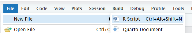 and save it
Package loading
We’ll use two main package, and two helpers. Our main packages are:
- DBI, which provides several ways of creating and accessing databases from R
- RSQLite, which contains the SQLite engine that (behind the scenes) has been powering our databases in the earlier sessions of this course
- palmerpenguins to give us some play data:
- glue to help us build up more complex queries
As a beginner, it can be hard to understand what DBI is doing, and what RSQLite is doing. To help explain, we’ll namespace functions in this introductory part, using the package::function notation to help keep clear what’s doing what. In ordinary practice I probably wouldn’t bother to do that because it makes the code a bit harder to read, but here I think the clarity it’s worth the extra lexical effort.
Create a database
That does a couple of things:
- the side-effect of that expression is to:
- check for the existence, and then create, a database file called
pengs.sqlitein your project root directory (check to see it exists) - then sets up the SQLite driver - think of this as the infrastructure to present that new database file as an SQL database
- finally, via
DBI::dbConnect, to create a connection to that SQLite database
- check for the existence, and then create, a database file called
- the return value of that expression is connection information for that database, which you should be able to see by inspecting the
pengs_dbobject you’ve just created
You can also create a temporary in-memory db by naming your connect :memory: which is worth knowing if you’re just doing a bit of play or practice.
Connecting to an existing SQLite database is very straightforward. If you’re working from a local file, just supply the path of the database file. If you were connecting to another SQL source, you would do your authentication etc inside DBI::dbConnect.
Add some tables to that database
pengs_db |>
  DBI::dbWriteTable("pengs_tbl", penguins) # table name, then R object name
As we’ll see below, writing SQL queries in R can make for some very complicated lines of code. I’ll use the base-R pipe |> to join lines of code here to cut down on that complexity. There’s nothing wrong with writing bracketed code though if you’re doing something simple - just make sure your connection is the first argument supplied to the DBI function:
# non-pipe
DBI::dbWriteTable(pengs_db, "pengs_tbl", penguins, overwrite = T) # without the overwrite this would fail as DBI has sensible default way of preventing you overwriting your tables
Write a query and try it
The most basic way of writing a query is to put the whole SQL query into the body of dbGetQuery:
pengs_db |>
DBI::dbGetQuery('SELECT species, island FROM pengs_tbl WHERE bill_depth_mm > 21')| species | island |
|---|---|
| Adelie | Torgersen |
| Adelie | Torgersen |
| Adelie | Torgersen |
| Adelie | Dream |
| Adelie | Dream |
| Adelie | Biscoe |
That’s assignable, so you should be able to easily capture that data once you’re satisfied your query works properly:
pengs_from_sql <- pengs_db |>
  DBI::dbGetQuery('SELECT species, island FROM pengs_tbl WHERE bill_depth_mm > 21')
pengs_from_sql # from the R object| species | island |
|---|---|
| Adelie | Torgersen |
| Adelie | Torgersen |
| Adelie | Torgersen |
| Adelie | Dream |
| Adelie | Dream |
| Adelie | Biscoe |
You’d use single quotes to build your query, because SQL column names might require escaping in R, and you’d use double quotes for that escaping. Building up a complex query as a single line of R code can be a challenge, and we’ll look at two ways of simplifying the process of writing more complex queries later in the session.
It’s also worth thinking a bit about what DBI::dbGetQuery is doing, which is to first run the query on our database, and then return the results as a data frame. Those steps can be taken independently too using DBI::dbSendQuery() to run the query, and DBI::dbFetch() to return any results. Being able to access these functions is especially helpful when you’re trying to modify a database in place, although note that’s a bit beyond the scope of this session. It’s also helpful when dealing with objects where the return values are uncomfortably large, especially when they wouldn’t fit as R objects in memory. There’s a neat method in the RSQLite vignette which shows how large objects can be fetched in pieces:
rs <- pengs_db |>
  dbSendQuery('SELECT * FROM pengs_tbl') # also worth showing that you can save a query as an R object

while (!dbHasCompleted(rs)) {
  df <- rs |>
    dbFetch(n = 100)  # n = number of rows/records per batch

  print(paste("That's grabbed", nrow(df), "rows of data this time round  \n")) # or whatever operation you actually want to do on the data
}
That’s grabbed 100 rows of data this time round
That’s grabbed 100 rows of data this time round
That’s grabbed 100 rows of data this time round
That’s grabbed 44 rows of data this time round
Disconnect from your database
pengs_db |>
  DBI::dbDisconnect()
You should then re-connect:
Getting more fancy with queries: parameters
pengs_db |>
  DBI::dbGetQuery('SELECT * FROM pengs_tbl WHERE year < :x LIMIT :y',
params = list(x = 2008, y = 5))| species | island | bill_length_mm | bill_depth_mm | flipper_length_mm | body_mass_g | sex | year |
|---|---|---|---|---|---|---|---|
| Adelie | Torgersen | 39.1 | 18.7 | 181 | 3750 | male | 2007 |
| Adelie | Torgersen | 39.5 | 17.4 | 186 | 3800 | female | 2007 |
| Adelie | Torgersen | 40.3 | 18.0 | 195 | 3250 | female | 2007 |
| Adelie | Torgersen | NA | NA | NA | NA | NA | 2007 |
| Adelie | Torgersen | 36.7 | 19.3 | 193 | 3450 | female | 2007 |
There’s a lot of clockwork to explore here (e.g. the dbBind function) - but for my money most of this would be better done with purrr or similar.
Getting more fancy with queries: glue
We mentioned before that SQL queries often need some kind of escaping from R. glue::glue_sql is a safe and easy way of doing that. Imagine that you’ve got a couple of R variables:
year <- 2008

group <- "island"

species <- "Adelie"
Rather than trying to paste those together, use glue::glue_sql, with each variable inside {}:
query <- glue::glue_sql("SELECT * from pengs_tbl WHERE species = {species} LIMIT 10", .con = pengs_db)DBI::dbGetQuery(pengs_db, query)| species | island | bill_length_mm | bill_depth_mm | flipper_length_mm | body_mass_g | sex | year |
|---|---|---|---|---|---|---|---|
| Adelie | Torgersen | 39.1 | 18.7 | 181 | 3750 | male | 2007 |
| Adelie | Torgersen | 39.5 | 17.4 | 186 | 3800 | female | 2007 |
| Adelie | Torgersen | 40.3 | 18.0 | 195 | 3250 | female | 2007 |
| Adelie | Torgersen | NA | NA | NA | NA | NA | 2007 |
| Adelie | Torgersen | 36.7 | 19.3 | 193 | 3450 | female | 2007 |
| Adelie | Torgersen | 39.3 | 20.6 | 190 | 3650 | male | 2007 |
| Adelie | Torgersen | 38.9 | 17.8 | 181 | 3625 | female | 2007 |
| Adelie | Torgersen | 39.2 | 19.6 | 195 | 4675 | male | 2007 |
| Adelie | Torgersen | 34.1 | 18.1 | 193 | 3475 | NA | 2007 |
| Adelie | Torgersen | 42.0 | 20.2 | 190 | 4250 | NA | 2007 |
Note (by inspecting that query object in your environment) that glue will as a default escape character values it receives from R. If you want to use those values as e.g. column names, unescape them with backticks - like {x}:
query <- glue::glue_sql("SELECT {`group`}, AVG(bill_length_mm) AS bill_length_{year} FROM pengs_tbl WHERE year == {year} GROUP BY {`group`}", .con = pengs_db)DBI::dbGetQuery(pengs_db, query)| island | bill_length_2008 |
|---|---|
| Biscoe | 44.62031 |
| Dream | 43.75588 |
| Torgersen | 38.76875 |
That opens the way to lots of areas of fun and interest, like building functions to pull data from an SQL query:
grab_pengs <- function(group = "species", year = 2007){
  query <- glue::glue_sql("SELECT {`group`}, AVG(bill_length_mm) AS bill_length_{year} FROM pengs_tbl WHERE year == {year} GROUP BY {`group`}", .con = pengs_db)

DBI::dbGetQuery(pengs_db, query)
}grab_pengs()| species | bill_length_2007 |
|---|---|
| Adelie | 38.82449 |
| Chinstrap | 48.72308 |
| Gentoo | 47.01471 |
grab_pengs(group = "island")| island | bill_length_2007 |
|---|---|
| Biscoe | 45.03864 |
| Dream | 44.53913 |
| Torgersen | 38.80000 |
There’s an odd * shorthand to vectorise:
DBI::dbGetQuery(pengs_db, qq)| island | species | bill_length |
|---|---|---|
| Biscoe | Adelie | 38.97500 |
| Biscoe | Gentoo | 47.50488 |
| Dream | Adelie | 38.50179 |
| Dream | Chinstrap | 48.83382 |
| Torgersen | Adelie | 38.95098 |