R beginner’s club 2024-06-13

Authors

Affiliation

KIND Network members

Brendan Clarke

NHS Education for Scotland

Published

September 20, 2024

How to compare two (or more) Excel spreadsheets?

The basic recipe here is:

read our Excel spreadsheets into R
try some simple base-R methods of comparison
get more fancy with packages for more useful comparisons

Reading in Excel files

This can be messy. readxl is probably the most straightforward place to start. Make sure a) that your Excel files aren’t open in Excel when you try to read them and b) that you’re happy and confident that your data is on the first worksheet (or you know the correct name of the sheet). You’ll almost certainly want to be working in an R project too to avoid too much messing around with file paths, getwd(), etc.

library(readxl) # to attach the readxl package
b1 <- read_xlsx("data/Book1.xlsx") 
b2 <- read_xlsx("data/Book2.xlsx") # to read the files

Basic comparisons

The most obvious thing to try first is a check for equality. You’ll do this with a double equal sign, like this:

b1 == b2

      name score
 [1,] TRUE  TRUE
 [2,] TRUE  TRUE
 [3,] TRUE  TRUE
 [4,] TRUE  TRUE
 [5,] TRUE  TRUE
 [6,] TRUE  TRUE
 [7,] TRUE  TRUE
 [8,] TRUE  TRUE
 [9,] TRUE  TRUE
[10,] TRUE  TRUE

(single = is effectively the same as <-)

That gives us back quite a complicated matrix of results, showing a cell-by-cell comparison of the two sets of data. This happens because R is vectorised - so when we compare two identically-shaped bits of data, R will assume that we want to do our comparison to each of the items in turn. If we just looked at the number values in our spreadsheets, which we could do by using the $ to refer to a column, we could:

b1$score - b2$score

 [1] 0 0 0 0 0 0 0 0 0 0

Which I suppose is another way of checking for equality. So could also use a helper function to collapse all of those down into one:

sum(b1$score - b2$score)

[1] 0

If we just wanted a simple true/false measure for the data as a whole, we could recruit the very useful all() and any():

all(b1 == b2) # to check all values are the same

[1] TRUE

any(b1 == b2) # to check any values are the same

[1] TRUE

You could do something very similar using setequal():

setequal(b1, b2)

[1] TRUE

More interesting comparisons

waldo::compare() is a brilliant way of comparing complex data:

waldo::compare(b1, b2)

✔ No differences

If we vandalise one of our datasets by changing one value, waldo does plenty of useful work to bring the correct parts of the data to our attention:

b2[5,2] <- 1
waldo::compare(b1, b2)

old vs new
                score
  old[2, ]  0.2481382
  old[3, ]  0.6444191
  old[4, ]  0.8873743
- old[5, ]  0.3361401
+ new[5, ]  1.0000000
  old[6, ]  0.1597596
  old[7, ]  0.3928778
  old[8, ]  0.5743370

`old$score[2:8]`: 0.2 0.6 0.9 0.3 0.2 0.4 0.6
`new$score[2:8]`: 0.2 0.6 0.9 1.0 0.2 0.4 0.6

I suppose we could also graph our data to show changed points. One way of doing this is to plot the two sets in different colours:

library(ggplot2)

ggplot() +
  geom_point(data = b1, aes(x = name, y = score), colour = "red", size = 5) +
  geom_point(data = b2, aes(x = name, y = score), colour = "blue", size = 5)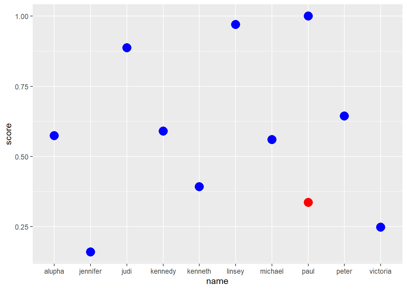

Or, possibly more elegantly, we could join our data using dplyr, then subtract one from the other, then plot the difference:

library(dplyr)

b1 |>
  left_join(b2, by = "name") |>
  ggplot(aes(x = name, xend = name, y = score.y - score.x, yend = 0), colour = "red") +
  geom_segment() +
  geom_label(aes(label = name))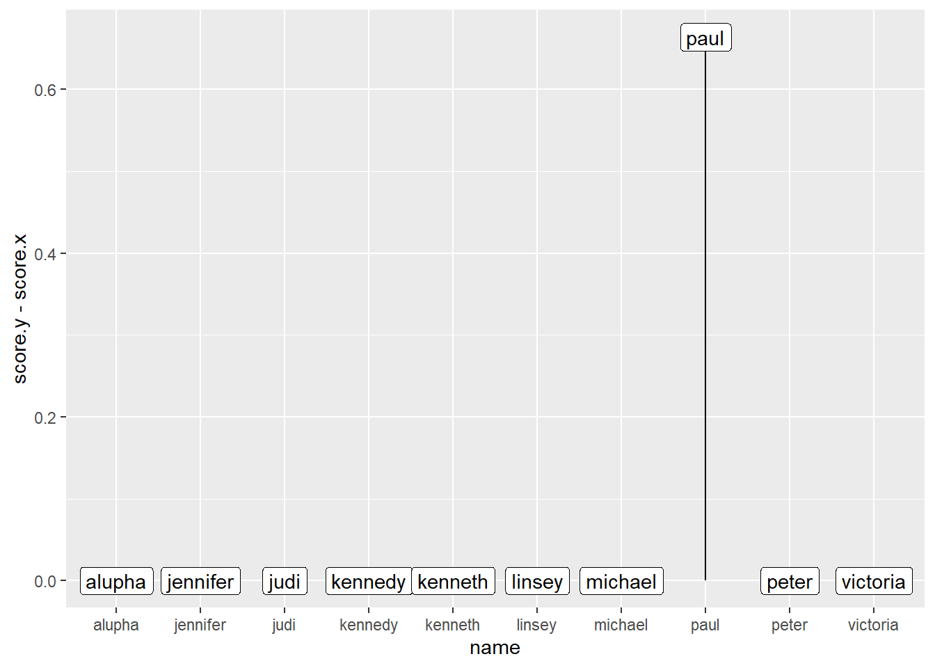

How to think about joins?

We did a simple join above. A join is a way of merging two datasets. Let’s demonstrate with some cut-down datasets from above. We’ll remove some of the values from our b1 set and from our b2 set:

b1 <- b1 |>
  slice(1:5)

b1

# A tibble: 5 × 2
  name     score
  <chr>    <dbl>
1 kennedy  0.590
2 victoria 0.248
3 peter    0.644
4 judi     0.887
5 paul     0.336

b2 <- b2 |>
  slice_sample(n = 5)

b2

# A tibble: 5 × 2
  name    score
  <chr>   <dbl>
1 kenneth 0.393
2 kennedy 0.590
3 peter   0.644
4 michael 0.561
5 judi    0.887

The simplest join we could do is to bind the rows from one set onto another:

b1 |>
  bind_rows(b2)

# A tibble: 10 × 2
   name     score
   <chr>    <dbl>
 1 kennedy  0.590
 2 victoria 0.248
 3 peter    0.644
 4 judi     0.887
 5 paul     0.336
 6 kenneth  0.393
 7 kennedy  0.590
 8 peter    0.644
 9 michael  0.561
10 judi     0.887

That just brings all the rows from b2 onto the end of b1. Unlike binding, though, in a join we usually want to only include some of our values. So let’s now left-join b2:

b1 |>
  left_join(b2, by = "name")

# A tibble: 5 × 3
  name     score.x score.y
  <chr>      <dbl>   <dbl>
1 kennedy    0.590   0.590
2 victoria   0.248  NA    
3 peter      0.644   0.644
4 judi       0.887   0.887
5 paul       0.336  NA

You should see that only the values from b2’s score column that have a corresponding name in b1 get populated, and everything else gets filled with NAs. Here’s a nice introduction to the different kinds of join you can do in dplyr.