Summarising data with dplyr

intermediate

Published

June 11, 2025

No feedback found for this session

Session outline

This session is an 🌶🌶 intermediate practical designed for those with some R experience. The aim of this session is to do three things with dplyr:

show how to approach summarising data
explain how grouping works
show some simple summary functions

You might also like some of the other dplyr-themed practical sessions:

Setup

Let’s do a little bit of package loading, find some interesting data, and then start summarising things:

library(dplyr)
library(readr)
library(lubridate)
library(ggplot2)
library(NHSRdatasets)

Data loading

For the first half of the session, we’ll use a real dataset that shows deaths by socioeconomic deprivation. Full details on the PHS opendata page:

SMR_SIMD <- read_csv("https://www.opendata.nhs.scot/datastore/dump/e6849f09-3a5c-44c6-8029-260882345071?bom=True") |>
  select(-c(`_id`, contains("QF"), Country)) |>
  tidyr::separate_wider_delim(TimePeriod, "Q", names = c("Year", "Quarter")) |>
  mutate(Year = as.numeric(Year),
         Quarter = as.numeric(Quarter) * 3) |>
  mutate(Date = ymd(paste(Year, Quarter, "01"))) |>
  mutate(SIMDQuintile = case_when(SIMDQuintile == "1 - most deprived" ~ "1",
                                  SIMDQuintile == "5 - least deprived" ~ "5",
                                  TRUE ~ SIMDQuintile)) |>
  relocate(last_col())

Data preview

We’ll do a quick skim() of the data to help you get a better sense of it:

skimr::skim(SMR_SIMD)

Data summary
Name	SMR_SIMD
Number of rows	204
Number of columns	7
_______________________
Column type frequency:
character	1
Date	1
numeric	5
________________________
Group variables	None

Variable type: character

skim_variable	n_missing	complete_rate	min	max	empty	n_unique	whitespace
SIMDQuintile	34	0.83	1	1	0	5	0

Variable type: Date

skim_variable	n_missing	complete_rate	min	max	median	n_unique
Date	0	1	2016-09-01	2024-12-01	2020-10-16	34

Variable type: numeric

skim_variable	complete_rate	mean	sd	p0	p25	p50	p75	p100	hist
Year	1	2020.24	2.47	2016.00	2018.00	2020.00	2022.00	2024.00	▆▇▃▇▇
Quarter	1	7.68	3.36	3.00	6.00	9.00	12.00	12.00	▇▇▁▇▇
NumberOfDeaths	1	1144.20	563.69	7.00	1006.00	1286.00	1551.00	2057.00	▃▁▆▇▃
NumberOfPatients	1	35444.62	16914.91	490.00	33310.00	39724.50	45818.25	59076.00	▃▁▃▇▃
CrudeRate	1	3.02	0.81	1.04	2.72	3.04	3.42	5.58	▂▃▇▂▁

This dataset is especially good for practising summarising, because there are various different plausible groups that we might like to investigate in it - especially the intersection between SIMDQuintiles (indicating different levels of deprivation) with the various date-based year/season/month groups that might be of interest for health improvement work:

Example time-series

SMR_SIMD |>
  ggplot() +
  geom_line(aes(x = Date, y = NumberOfDeaths, colour = SIMDQuintile)) +
  theme_minimal()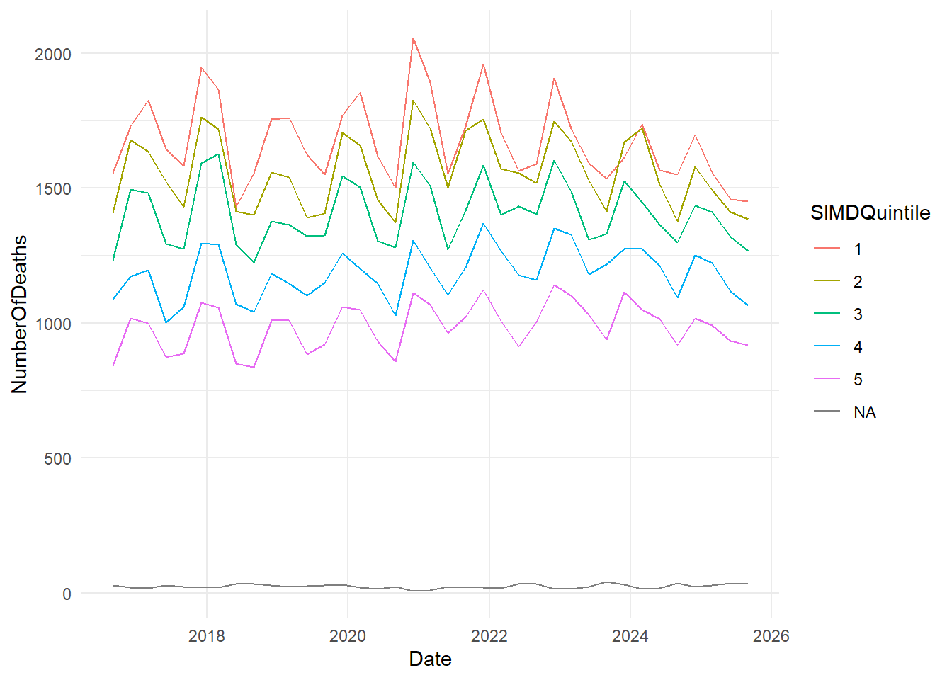

`summarise()`

This is the standard way of summarising data in dplyr. The description on the dplyr reference page for summarise is admirably clear:

summarise() creates a new data frame. It returns one row for each combination of grouping variables; if there are no grouping variables, the output will have a single row summarising all observations in the input. It will contain one column for each grouping variable and one column for each of the summary statistics that you have specified.

Basic example

SMR_SIMD |> 
  summarise(sum(NumberOfDeaths))

# A tibble: 1 × 1
  `sum(NumberOfDeaths)`
                  <dbl>
1                233417

`group_by()`

summarise() is especially strong in concert with group_by():

SMR_SIMD |> 
  group_by(Year) |>
  summarise(sum(NumberOfDeaths))

# A tibble: 9 × 2
   Year `sum(NumberOfDeaths)`
  <dbl>                 <dbl>
1  2016                 13273
2  2017                 27471
3  2018                 26670
4  2019                 26940
5  2020                 27717
6  2021                 28745
7  2022                 28101
8  2023                 27670
9  2024                 26830

Care with groups

Two important things to note here:

group_by doesn’t change how the data looks - just how it behaves:
Each call to summarise() removes a layer of grouping

SMR_SIMD |> 
  group_by(Year) |>
  summarise(sum(NumberOfDeaths)) |>
  summarise(sum(`sum(NumberOfDeaths)`)) # horrible default column names, which we'll fix in future

# A tibble: 1 × 1
  `sum(\`sum(NumberOfDeaths)\`)`
                           <dbl>
1                         233417

Renaming summary columns

You can build simple formulae inside summarise():

SMR_SIMD |> 
  group_by(Year) |>
  summarise(total = sum(NumberOfDeaths)) # rename columns like select or rename

# A tibble: 9 × 2
   Year total
  <dbl> <dbl>
1  2016 13273
2  2017 27471
3  2018 26670
4  2019 26940
5  2020 27717
6  2021 28745
7  2022 28101
8  2023 27670
9  2024 26830

Expressions within summaries

You can also build-up more complex expressions within summarise

SMR_SIMD |> 
  group_by(Year) |>
  summarise(surviving = sum(NumberOfPatients - NumberOfDeaths ))  #  mutate()-like expressions

# A tibble: 9 × 2
   Year surviving
  <dbl>     <dbl>
1  2016    447292
2  2017    888462
3  2018    885537
4  2019    919377
5  2020    662219
6  2021    737727
7  2022    778326
8  2023    832262
9  2024    846083

`by()`

You can, in another recent change, group inside the summarise itself via .by():

SMR_SIMD |> 
  summarise(surviving = sum(NumberOfPatients - NumberOfDeaths), 
            .by = Year)

# A tibble: 9 × 2
   Year surviving
  <dbl>     <dbl>
1  2016    447292
2  2017    888462
3  2018    885537
4  2019    919377
5  2020    662219
6  2021    737727
7  2022    778326
8  2023    832262
9  2024    846083

This always returns an ungrouped tibble - so important to know that it’s not a direct substitute for an ordinary group_by()…

`summarise()` removes one layer of grouping

The most confusing aspect of summarise() is that it removes the bottom layer of grouping each time. Here, we start with our data grouped by Year and Quarter. After summarising, the data is grouped by Year only.:

SMR_SIMD |> 
  group_by(Year, Quarter) |>
  summarise(att = sum(NumberOfDeaths)) |>
  group_vars()

[1] "Year"

Tools for understanding groupings

group_vars() is just one of a group of functions in dplyr for understanding grouping metadata. Let’s start with some simple grouped data. We can discover the groups that we’re working with using groups():

SMR_SIMD |> 
  group_by(Year) |>
  groups() # as a list

[[1]]
Year

`group_vars()`

Simpler information is produced by group_vars():

SMR_SIMD |> 
  group_by(Year) |>
  group_vars() # vector

[1] "Year"

`group_data()` etc

Much fuller information by group_data(), group_rows() and friends:

SMR_SIMD |> 
  group_by(Year) |>
  group_data() # tibble

# A tibble: 9 × 2
   Year       .rows
  <dbl> <list<int>>
1  2016        [12]
2  2017        [24]
3  2018        [24]
4  2019        [24]
5  2020        [24]
6  2021        [24]
7  2022        [24]
8  2023        [24]
9  2024        [24]

SMR_SIMD |> 
  group_by(Year) |>
  group_rows() # list of each group's rows

<list_of<integer>[9]>
[[1]]
 [1]  1  2  3  4  5  6  7  8  9 10 11 12

[[2]]
 [1] 13 14 15 16 17 18 19 20 21 22 23 24 25 26 27 28 29 30 31 32 33 34 35 36

[[3]]
 [1] 37 38 39 40 41 42 43 44 45 46 47 48 49 50 51 52 53 54 55 56 57 58 59 60

[[4]]
 [1] 61 62 63 64 65 66 67 68 69 70 71 72 73 74 75 76 77 78 79 80 81 82 83 84

[[5]]
 [1]  85  86  87  88  89  90  91  92  93  94  95  96  97  98  99 100 101 102 103
[20] 104 105 106 107 108

[[6]]
 [1] 109 110 111 112 113 114 115 116 117 118 119 120 121 122 123 124 125 126 127
[20] 128 129 130 131 132

[[7]]
 [1] 133 134 135 136 137 138 139 140 141 142 143 144 145 146 147 148 149 150 151
[20] 152 153 154 155 156

[[8]]
 [1] 157 158 159 160 161 162 163 164 165 166 167 168 169 170 171 172 173 174 175
[20] 176 177 178 179 180

[[9]]
 [1] 181 182 183 184 185 186 187 188 189 190 191 192 193 194 195 196 197 198 199
[20] 200 201 202 203 204

`reframe()`

A recent change in dplyr 1.1.0 is that summarise() now will only return one row per group. A new function, reframe(), has been developed to produce multiple-row summaries. It works exactly like summarise() except, rather than removing one grouping layer per operation, it always returns an ungrouped tibble. The syntax is the same as summarise():

sum <- ae_attendances |>
  group_by(year = lubridate::floor_date(period, unit = "year")) |>
  summarise(
    year = lubridate::year(year),
    non_admissions = sum(attendances - admissions)
  )

ref <- ae_attendances |>
  group_by(year = lubridate::floor_date(period, unit = "year")) |>
  reframe(
    year = lubridate::year(year),
    non_admissions = sum(attendances - admissions)
  )

waldo::compare(sum, ref)

`class(old)`: "grouped_df" "tbl_df" "tbl" "data.frame"
`class(new)`:              "tbl_df" "tbl" "data.frame"

`attr(old, 'groups')` is an S3 object of class <tbl_df/tbl/data.frame>, a list
`attr(new, 'groups')` is absent

`count()`

count() counts unique values, and is equivalent to using group_by() and then summarise():

synthetic_news_data |>
  count(died)

# A tibble: 2 × 2
   died     n
  <int> <int>
1     0   930
2     1    70

`count()` is a shorthand for grouping and summarising

That’s roughly equivalent to:

synthetic_news_data |> 
  group_by(died) |> 
  summarise(n = n())

# A tibble: 2 × 2
   died     n
  <int> <int>
1     0   930
2     1    70

`tally()`

tally() works similarly, except without the group_by():

synthetic_news_data |> 
  # group_by(died) |> 
  summarise(n = n())

# A tibble: 1 × 1
      n
  <int>
1  1000

synthetic_news_data |>
  tally()

# A tibble: 1 × 1
      n
  <int>
1  1000

Weighted counts

A possible source of confusion is that adding a column name to either count() or tally() performs a weighted count of that column:

synthetic_news_data |>
  tally(age) # totally dis-similar behaviour to count

# A tibble: 1 × 1
      n
  <int>
1 69647

Roughly equivalent to:

synthetic_news_data |>
  pull(age) |>
  sum()

[1] 69647

Named arguments

Personally, it seems wise to use named arguments inside count() and tally() to make sure it’s obvious what the column name is doing:

synthetic_news_data |>
  count(wt = age)

# A tibble: 1 × 1
      n
  <int>
1 69647

Sorting

count() has a useful sort option to arrange by group size:

synthetic_news_data |>
  count(syst, sort=T)

# A tibble: 125 × 2
    syst     n
   <int> <int>
 1   130    28
 2   120    26
 3   139    26
 4   150    25
 5   135    24
 6   126    22
 7   134    22
 8   119    21
 9   123    21
10   112    20
# ℹ 115 more rows

Controlling column names

And you can name your new count column something more descriptive than n:

synthetic_news_data |>
  count(syst, name = "count_of_something")

# A tibble: 125 × 2
    syst count_of_something
   <int>              <int>
 1    65                  2
 2    76                  2
 3    78                  1
 4    80                  6
 5    81                  1
 6    82                  2
 7    83                  1
 8    85                  5
 9    86                  2
10    87                  2
# ℹ 115 more rows

Empty groups

If you want to count empty groups, use .drop:

synthetic_news_data |>
  mutate(male = factor(male, levels = c(0, 1, 2))) |>
  count(male, .drop = T)

# A tibble: 2 × 2
  male      n
  <fct> <int>
1 0       524
2 1       476

synthetic_news_data |>
  mutate(male = factor(male, levels = c(0, 1, 2))) |>
  count(male, .drop = F)

# A tibble: 3 × 2
  male      n
  <fct> <int>
1 0       524
2 1       476
3 2         0

`add_count()`

Both count() and tally() have add_ variants, which work like mutate() in that they add a new column containing the count:

#add_ variants
synthetic_news_data |>
  add_count(syst, name="syst_BP_count") |>
  select(syst, last_col())

# A tibble: 1,000 × 2
    syst syst_BP_count
   <int>         <int>
 1   150            25
 2   145            16
 3   169             4
 4   154            12
 5   122            11
 6   146            16
 7    65             2
 8   116            12
 9   162            10
10   132             9
# ℹ 990 more rows

`add_tally()`

add_tally() gives a col with the same value in each row of a group:

synthetic_news_data |>
  group_by(died) |>
  add_tally() |>
  slice(1:3)

# A tibble: 6 × 13
# Groups:   died [2]
   male   age  NEWS  syst  dias  temp pulse  resp   sat   sup alert  died     n
  <int> <int> <int> <int> <int> <dbl> <int> <int> <int> <int> <int> <int> <int>
1     0    68     3   150    98  36.8    78    26    96     0     0     0   930
2     1    94     1   145    67  35      62    18    96     0     0     0   930
3     0    85     0   169    69  36.2    54    18    96     0     0     0   930
4     0    80     5   130    81  37     129    18    97     0     0     1    70
5     0    62     6   108    65  34.4    43    18    99     0     0     1    70
6     1    64     0   114    82  36.2    78    18    97     0     0     1    70

`rowwise()`

rowwise() forms groups per row. For example, we could take the average of the three columns in ae_attendances:

# to find the daily mean of attendances, breaches, and admissions
ae_attendances |> 
  rowwise() |>
  mutate(mean = mean(c(attendances, breaches, admissions)))

# A tibble: 12,765 × 7
# Rowwise: 
   period     org_code type  attendances breaches admissions   mean
   <date>     <fct>    <fct>       <dbl>    <dbl>      <dbl>  <dbl>
 1 2017-03-01 RF4      1           21289     2879       5060  9743.
 2 2017-03-01 RF4      2             813       22          0   278.
 3 2017-03-01 RF4      other        2850        6          0   952 
 4 2017-03-01 R1H      1           30210     5902       6943 14352.
 5 2017-03-01 R1H      2             807       11          0   273.
 6 2017-03-01 R1H      other       11352      136          0  3829.
 7 2017-03-01 AD913    other        4381        2          0  1461 
 8 2017-03-01 RYX      other       19562      258          0  6607.
 9 2017-03-01 RQM      1           17414     2030       3597  7680.
10 2017-03-01 RQM      other        7817       86          0  2634.
# ℹ 12,755 more rows

many dplyr verbs respect grouping

Compare and contrast with the results we obtain if we omit rowwise(), where the mean column contains the averages of the three columns overall, rather than for each date and organisation:

ae_attendances |> 
  mutate(mean=mean(c(attendances, breaches, admissions)))

# A tibble: 12,765 × 7
   period     org_code type  attendances breaches admissions  mean
   <date>     <fct>    <fct>       <dbl>    <dbl>      <dbl> <dbl>
 1 2017-03-01 RF4      1           21289     2879       5060 2450.
 2 2017-03-01 RF4      2             813       22          0 2450.
 3 2017-03-01 RF4      other        2850        6          0 2450.
 4 2017-03-01 R1H      1           30210     5902       6943 2450.
 5 2017-03-01 R1H      2             807       11          0 2450.
 6 2017-03-01 R1H      other       11352      136          0 2450.
 7 2017-03-01 AD913    other        4381        2          0 2450.
 8 2017-03-01 RYX      other       19562      258          0 2450.
 9 2017-03-01 RQM      1           17414     2030       3597 2450.
10 2017-03-01 RQM      other        7817       86          0 2450.
# ℹ 12,755 more rows

`c_across()`

There’s also a c_across() function to select columns that looks really promising for rowwise() work, but bafflingly it is extremely slow here, taking 50x longer than the equivalent mutate(). This is a known issue - “particularly for long, narrow, data”. So this code is switched off and provided here for information only - although do feel free to try it out if you don’t mind a ten second wait.

ae_attendances |> 
  rowwise() |>
  mutate(mean = mean(c_across(4:6)))

Summary functions: `nth()` / `first()` / `last()`

Get the nth, first, or last values. Very useful inside a summarise() or similar when you want to be sure that you’re going to return a sensible result.

tibble(speaker = c("steve", "steve", "emma", "steve", "emma", "emma"),
       comment = letters[1:6])  |>
  mutate(group = consecutive_id(speaker)) |>
  group_by(group, speaker) |>
  summarise(comment = last(comment)) |>
  ungroup() |>
  select(-group)

# A tibble: 4 × 2
  speaker comment
  <chr>   <chr>  
1 steve   b      
2 emma    c      
3 steve   d      
4 emma    f

Acknowledgments

I’m extremely grateful to Pauline Ward (PHS) for suggesting the dataset used for this session.

Session outline

Setup

Data loading

Data preview

Example time-series

summarise()

Basic example

group_by()

Care with groups

Renaming summary columns

Expressions within summaries

by()

summarise() removes one layer of grouping

Tools for understanding groupings

group_vars()

group_data() etc

reframe()

count()

count() is a shorthand for grouping and summarising

tally()