No feedback found for this session
Scope of the possible with R
R
overview
Welcome
- this session is a non-technical overview designed for service leads
Session outline
- Introducing R, and a bit of chat about the aims of this session
- Practical demo - take some data, load, tidy, analyse, produce outputs
- Strengths and weaknesses
- obvious
- less obvious
- Alternatives
- Skill development
Introducing R
- free and open-source statistical programming language
- multi-platform
- large user base
- prominent in health, industry, biosciences
Why this session?
- R can be confusing
- it’s code-based, and most of us don’t have much code experience
- it’s used for some inherently complicated tasks
- it’s a big product with lots of add-ons and oddities
- But R is probably the best general-purpose toolbox we have for data work at present
- big user base in health and social care
- focus on health and care-like applications
- not that hard to learn
- extensible and flexible
- capable of enterprise-y, fancy uses
- yet there’s signficant resistant to using R in parts of Scotland’s health and care sector
R demo
- this is about showing what’s possible, and give you a flavour of how R works
- we won’t explain code in detail during this session
- using live open data
Hello world!
There are lots of ways to run R. In this session, we’ll demonstrate using the Rstudio Desktop IDE on Windows.
"Hello world!"[1] “Hello world!”
Packages
R is highly extensible using packages: collections of useful code
Create variables
url <- "https://www.opendata.nhs.scot/dataset/0d57311a-db66-4eaa-bd6d-cc622b6cbdfa/resource/a5f7ca94-c810-41b5-a7c9-25c18d43e5a4/download/weekly_ae_activity_20251123.csv"Load some open data
That’s a link to data about weekly A+E activity. It’s large-ish (approximately 40000 rows)
ae_activity <- read_csv(url)One small bit of cheating: renaming
Preview
| date | country | hb | loc | type | attend | n | n_in_4 | n_4 | perc_4 | n_8 | perc_8 | n_12 | perc_12 |
|---|---|---|---|---|---|---|---|---|---|---|---|---|---|
| 20220828 | S92000003 | S08000026 | Z102H | Type 1 | New planned | 4 | 3 | 1 | 75.0 | 0 | 0.0 | 0 | 0 |
| 20190602 | S92000003 | S08000024 | S319H | Type 1 | All | 964 | 911 | 53 | 94.5 | 1 | 0.1 | 0 | 0 |
| 20171112 | S92000003 | S08000022 | C121H | Type 1 | All | 136 | 136 | 0 | 100.0 | 0 | 0.0 | 0 | 0 |
| 20190714 | S92000003 | S08000031 | G107H | Type 1 | All | 1928 | 1555 | 373 | 80.7 | 10 | 0.5 | 0 | 0 |
| 20170611 | S92000003 | S08000030 | T202H | Type 1 | All | 474 | 469 | 5 | 98.9 | 0 | 0.0 | 0 | 0 |
Removing data
| date | hb | loc | type | attend | n | n_in_4 | n_4 | n_8 | n_12 |
|---|---|---|---|---|---|---|---|---|---|
| 20220807 | S08000031 | G513H | Type 1 | All | 1214 | 1192 | 22 | 0 | 0 |
| 20171015 | S08000030 | T202H | Type 1 | All | 440 | 436 | 4 | 0 | 0 |
| 20191013 | S08000031 | C418H | Type 1 | Unplanned | 1316 | 1013 | 303 | 56 | 5 |
| 20241124 | S08000017 | Y144H | Type 1 | All | 253 | 216 | 37 | 3 | 0 |
| 20240303 | S08000015 | A210H | Type 1 | All | 601 | 409 | 192 | 111 | 79 |
Tidying data
| date | hb | loc | type | attend | n | n_in_4 | n_4 | n_8 | n_12 |
|---|---|---|---|---|---|---|---|---|---|
| 2022-02-20 | S08000016 | B120H | Type 1 | All | 616 | 405 | 211 | 101 | 69 |
| 2023-09-24 | S08000015 | A111H | Type 1 | All | 1194 | 834 | 360 | 158 | 91 |
| 2017-10-22 | S08000017 | Y146H | Type 1 | Unplanned | 656 | 591 | 65 | 1 | 0 |
| 2018-06-17 | S08000026 | Z102H | Type 1 | Unplanned | 171 | 164 | 7 | 0 | 0 |
| 2022-01-30 | S08000032 | L302H | Type 1 | New planned | 8 | 8 | 0 | 0 | 0 |
Subset data
We’ll take a selection of 5 health boards to keep things tidy:
boards_sample <- c("NHS Borders", "NHS Fife", "NHS Grampian", "NHS Highland", "NHS Lanarkshire")Joining data
Those board codes (like S08000020) aren’t very easy to read. Luckily, we can add the proper “NHS Thing & Thing” board names from another data source.
boards <- read_csv("https://www.opendata.nhs.scot/dataset/9f942fdb-e59e-44f5-b534-d6e17229cc7b/resource/652ff726-e676-4a20-abda-435b98dd7bdc/download/hb14_hb19.csv")| HB | HBName | HBDateEnacted | HBDateArchived | Country |
|---|---|---|---|---|
| S08000030 | NHS Tayside | 20180202 | NA | S92000003 |
| S08000022 | NHS Highland | 20140401 | NA | S92000003 |
| S08000023 | NHS Lanarkshire | 20140401 | 20190331 | S92000003 |
| S08000018 | NHS Fife | 20140401 | 20180201 | S92000003 |
| S08000026 | NHS Shetland | 20140401 | NA | S92000003 |
We can do something very similar with the A&E locations:
And we can add the postcodes:
We can then join our three datasets together to give us data with the NHS Board names, A&E names, and locations:
| date | HBName | loc | type | n | n_in_4 | n_4 | n_8 | n_12 | loc_name | postcode | long | lat |
|---|---|---|---|---|---|---|---|---|---|---|---|---|
| 2024-09-08 | NHS Lanarkshire | L302H | Type 1 | 1253 | 746 | 507 | 139 | 52 | University Hospital Hairmyres | G75 8RG | -4.221963 | 55.75982 |
| 2017-10-29 | NHS Highland | H212H | Type 1 | 160 | 153 | 7 | 0 | 0 | Belford Hospital | PH336BS | -5.104701 | 56.81941 |
| 2016-08-21 | NHS Highland | H103H | Type 1 | 138 | 128 | 10 | 1 | 0 | Caithness General Hospital | KW1 5NS | -3.095744 | 58.44133 |
| 2017-10-22 | NHS Borders | B120H | Type 1 | 575 | 551 | 24 | 1 | 0 | Borders General Hospital | TD6 9BS | -2.741945 | 55.59548 |
| 2020-11-08 | NHS Lanarkshire | L106H | Type 1 | 1008 | 782 | 226 | 54 | 9 | University Hospital Monklands | ML6 0JS | -3.999588 | 55.86588 |
Basic plots

Looking across different measures
library(tidyr)

ae_activity_locs |>
  filter(loc_name == "Raigmore Hospital") |>
  select(date, n_in_4:n_12) |>
  pivot_longer(-date) |>
  group_by(date = floor_date(date, "month"), name) |>
  summarise(value = mean(value)) |>
  ggplot(aes(x = date, y = value, colour = name)) +
  geom_line() +
  geom_smooth(se = F)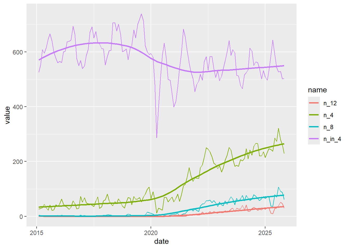
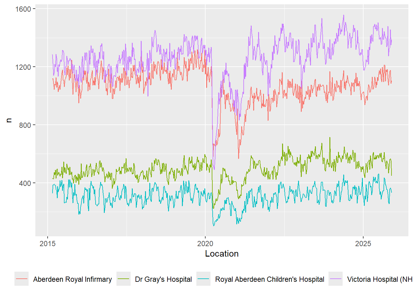
Making that re-usable
A rubbish map
We’ve got latitude and longitude information for our A&E sites, which means we can plot them on a map:
ae_activity_locs |>
  ggplot(aes(x = long, y = lat, label = loc_name, colour = HBName)) +
  geom_point() +
  theme_void() +
  theme(legend.position = "none")
That’s not the most useful map I’ve ever seen. Luckily, there’s a package to help us:
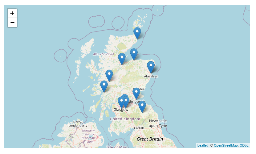
Add to a map
ae_activity_locs |>
    leaflet::leaflet() |>
    leaflet::addTiles() |>
    leaflet::addMarkers(~long, ~lat, label = ~loc_name)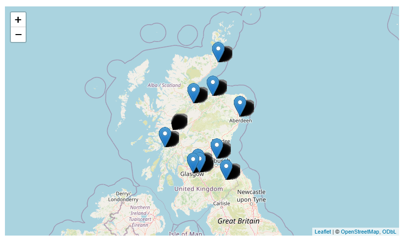
Then make that map more useful
Strengths
R offers enormous scope and flexibility, largely because of two features. First, R is based on the idea of packages, where you’re encouraged to outsource specialist functions to your R installation in a repeatable and standard way. There’s basically a package for everything - something over 20000 at present. Second, R encourages reproducible analytics: the idea being you write your script once, and then run it many times as your data changes, producing standardised outputs by design.
Together, that design makes R a force-multiplier for fancier data work: use packages to replicate your existing work in a reproducible way, then use the time saved in your routine reporting to improve and extend the work. There are other features of code-based analytics which make collaborating and developing more complex projects typically much smoother than they would be in non-code tools like Excel.
Weaknesses
- it’s code, and it takes some time (months to years) to achieve real fluency
- potentially harder to learn than some competitor languages and tools (Power BI, Python)
- very patchy expertise across H+SC Scotland
- complex IG landscape
- messy skills development journey